2.2 Estimating Economic Lifecycle

Introduction

The following steps apply to estimating the age profiles of consumption and labor income.

Estimate the per capita age-profile for the variable using individual/household survey data or administrative records.
Use population data to construct a preliminary aggregate age-profile.
Adjust the per capita profiles to match aggregate controls.

Age profiles are estimates of per capita values by single year of age. We assume that all consumption within the household and that all public consumption can be assigned to individuals. Likewise, we assume that the value of labor income can be assigned to individuals working in firms or in family enterprise. This assumes away pure public goods, economies of scale, and other important features of consumption and production.

The data that are available will vary from country to country and, consequently, the methods employed will vary. In some instances, data on variables of interest are collected for individuals and per capita profiles can be directly tabulated. This is not usually the case, however. Often statistical techniques or simple rules are used to allocate data reported for households to the individuals residing in the household.

Once this is accomplished per capita profiles can be tabulated from the available survey data. Note that appropriate sample weights should be used in all cases. The per capita age profiles are noisy, particularly at ages with relatively few observations, and hence the NTA variables should be smoothed with important exceptions explained below.

The next step is to adjust the per capita age profiles to match the aggregate control as explained above. Population data is needed to construct a preliminary aggregate age-profile. Then we use the aggregate profile and the per capita profile to match a control total taken from NIPA or some other source.

Consumption

Consumption is equal to private consumption plus public consumption. These are explained in turn.

Private Consumption

Introduction

Private consumption is the value of goods and services consumed by individuals, households, or NPISHs that are acquired through the private sector. We assume that all consumption can be assigned to individuals. This assumes away pure public goods, economies of scale, and other important features of consumption and production.

Private consumption is typically allocated to individuals based on household surveys. The methods described here assume the availability of one or more household surveys which include detailed expenditure data for the household and the number and age of all household members. Ideally the surveys are nationally representative.

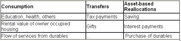
Household expenditure surveys usually include all household expenditures or outflows. Although only consumption expenditures are needed to estimate consumption age profiles, other outflows are used to estimate other NTA components. Thus, it is useful to classify all household expenditures or outflows during the year as falling into one of three categories - consumption, transfers, or asset-based reallocations:

Priv C

NTA methodology distinguishes three components of private consumption: education, health, and other consumption. Education and health are estimated separately because they vary substantially by age.

Private education consumption includes tuition, books and fees, school supplies for all school levels including pre-school and tutoring expenses. The exact definition will vary depending on data availability. In Taiwan, for example, reference materials and self-improvement classes (art classes, music classes, etc.) are also included.

Private health consumption includes out-of-pocket health expenditure and reimbursement to health providers by private health insurance companies. If firms provide medical services directly to their employees and their dependents, the value of these services are also included in private health consumption. It is important to note that there are differences between NIPA and NTA, and between NIPA and National Health Account (NHA).

Other consumption includes housing consumption for owner-occupants, that is, the value of the annual services that home yields typically measured as the amount for which the home could be rented. The purchase of a home is a component of saving and investment. Consumer durables should be treated, in principle, in the same way as housing. Consumption is the value of the services from the durables. The purchase of the durable is then classified as saving. Household expenditure surveys typically report the rental value of owner occupied housing. Whether or not consumption of durables can be measured as a flow rather than a purchase will vary from country to country. If data on durable ownership are not available, the purchase of durables is treated as consumption.

The following items should be classified as transfers and not included in consumption: tax payments, gifts, remittances, donations, and similar items.

The following items are classified as asset-based reallocations and not included in consumption: the purchase of a home; the purchase of consumer durables, the purchase of stocks, bonds, and other securities; investment in a business or farm; increases in cash holdings; interest payments; rent on land. Expenditure surveys will vary in the extent to which these items are reported. Often saving is estimated as a residual, i.e., income plus net transfers less consumption.

Some items require particular attention although they may be unimportant in some countries or data may limit the extent to which they can be treated.

Insurance: Some insurance premiums (whole life insurance) are a form of saving. Consumers pay a premium and their policy accrues value that can be cashed in at a later date or borrowed against. This is saving. Other forms of insurance provide consumers with a way of pooling risk. Term life insurance and property and casualty insurance are examples of these forms of insurance. Some portion of premiums collected each year are paid to beneficiaries who have experienced the particular event being insured. These payments are transfers. Although they may produce inter-age reallocations, we assume that premiums are assessed in an actuarially fair way and, hence, produce only intra-age reallocations. Hence, they are not included in NTA. The remaining portion of premiums paid by consumers for the administrative costs and profits of insurance companies represents the cost and value of the risk-pooling services provided by insurance. It is classified as consumption by NIPA and by NTA.

The US NIPA has recently been revised because catastrophic losses, e.g., those produced by Hurricane Katrina, lead to large fluctuations in insurance related components. The new revisions measure the consumption of insurance services using an estimate of normal profits. Catastrophic losses that lead to actual profits that differ from normal profits are treated as a transfer.

Health: In NIPA private health consumption includes the value of all goods and services that are marketed, i.e., goods and services purchased from either private or public providers. Public health consumption includes only goods and services that are provided as in-kind transfers. Examples are the subsidized portion of public inoculation programs, public sanitation programs, free clinics, family planning programs, etc. Private consumption includes goods and services purchased and reimbursed through public cash transfer programs. Health consumption reimbursed by Medicare and Medicaid in the US and by National Health Insurance in Taiwan are classified as private health consumption in NIPA. However, in NTA, private health consumption that is reimbursed by the public sector is re-classified as public health consumption.

There are also important differences between NIPA and the NHA that should be kept in mind. First, NHA document expenditures rather than consumption. Expenditure is a broader measure that does not distinguish consumption from investment and profits. Private health expenditure, for example, includes the profits of insurance companies. Second, public national health expenditure in NHA includes both in-kind and cash transfers.

Separate procedures are used to allocate education, health, and housing and other consumption to household members. The methods described here are intended as illustrative and should be adapted to the particular circumstances of the country being analyzed and to the particular data that are available. The method of choice is to rely on individual level data for any consumption component, but these are rarely available.

Private Education Consumption

Education is typically allocated using a regression model. The household consumption of education (CFEj) is,

${CFE}_j= \sum_a \alpha (a) E_j(a) + \sum_a \beta (a) {NE}_j(a)+\epsilon_j$

where ${E}_j$ is the number of enrolled members aged a (single age) in household j, and ${NE}_j$ is the number of not enrolled members aged a in household j. The number of members not enrolled captures educational spending that is not part of the formal educational system. Note that this equation is estimated in homogeneous form (without an intercept) insuring that household consumption is fully allocated.

The survey usually identifies who is enrolled and who is not in each household. If the information is not available, then each country team decides these age groups, based on the country’s schooling system. The age groups included varies with the country and with enrollment rates. In Taiwan, the number of enrolled includes those aged 3 to 29, although it varies by year.

The regression method may yield negative coefficients for some age groups with very low or no enrollments. If so, the negative coefficients should be replaced with zero to avoid negative expenditure.

The regression estimates are used to allocate the education expenditure for each household j to household member i. For example, for those who are enrolled:

${CFE}_i_j (x)= {CFE}_j\alpha(x) / \sum_a \alpha(a) {E}_j(a)$

where x is the age of the ith household member. Education consumption for those not enrolled is calculated in similar fashion. Stata programming code for Taiwan is available in the Appendix section.

Education consumption is intrinsically not smooth and the best approach is often to use the unsmoothed age profile to construct final estimates. Some smoothing at older ages may be warranted, however. Smoothing is discussed below.

Private Health Consumption

The allocation of private health consumption is difficult because of the complex ways in which it is financed. Three sources of finance are important in many countries: private out-of-pocket expense, private insurance, and the public sector. Different age allocation methods may be required for each of these components of health consumption.

National Health Accounts (NHA), available in some countries, provide a useful breakdown by source of finance.

The method used to allocate health varies depending on the availability of data.

Age profile of individual utilization measures. In some cases the expenditure survey may include utilization measures for household members. In this case, a model similar to the model employed for education can be used. For example, household health expenditure can be regressed on the number of members using outpatient services in each age group and the number of members using inpatient services in each age group. That is, the household consumption (CFHj) is regressed on the number of inpatients and outpatients aged a in each household:

${CFH}_j= \sum_a \alpha(a) {IN}_j(a)+\sum_a \beta(a) {OUT}_j(a) + \epsilon_j$

Stata programming code for Taiwan is available in the Appendix section.

Age profile of utilization from alternative source. In some countries, such as Japan, per capita utilization by age is available from alternative sources. The household health consumption estimated is:

${CFH}_j= \sum_a \beta(a) U(a)M_j(a) + \epsilon_j$

where U(a) represents a single utilization measure for each age, and Mj(a) is the number of household members aged a in household j. The estimated parameters $\beta(a)$ are interpreted as the unit cost for each age. In some cases it may be reasonable to assume that the unit cost is independent of age, but this is probably an unattractive option for health services. Thus, the unit cost may be assumed to be quadratic in age, for example. In this case, the model to be estimated is:

${CFH}_j= \sum_a \beta_0(a) U(a)M_j(a) + \sum_a \beta_1(a) U(a)M_j(a)+ \sum_a \beta_2 a^2 U(a)M_j(a) + \epsilon_j$

As with the education method presented above, the estimated model is used to “predict” health expenditure for persons aged a. In this case, the predicted cost would be:

$\hat{\beta}_0 U(a) + \hat{\beta}_1 U(a) + \hat{\beta}_2 {a}^2 U(a)$

The predicted costs are used to allocate the observed health expenditure in each household to individual members. Then the health expenditures are tabulated to construct the per capita profile.

Iterative Method. This approach works by assigning health expenditure equally to each household member and then tabulating the per capita profile. The per capita profile is then used as weights to allocate health expenditure to household members producing a new per capita profile. The procedure can be repeated each time using the newly generated profile to allocate household expenditure. Under some conditions, this approach will converge to the actual underlying profile. Whether it will always do so is unknown at this point. An attractive feature of this method is that negative values will not be generated.

Simple Regression Approach. This approach is not recommended unless absolutely nothing else is possible. The regression approach used for health differs from the model used for education because there is no variable that capture which individuals are receiving health care services. Hence, household health expenditure is regressed on the number of household members in each age group ${M}_j(a)$

${CFH}_j= \sum_a \beta(a) M_j(a) + \epsilon_j$

The age groups can be single year or broader age groups.

Private Other Household Consumption

All other household consumption is allocated to individuals using an ad hoc allocation rule based on an extensive review of the literature on household consumption. Evaluation of other methods, e.g., Engel’s method and the Rothbarth method, has shown them to be unreliable and we do not recommend that they be used.

Consumption of individuals living within any household j is assumed to be proportional to an equivalence scale that is equal to 1 for adults aged twenty or older, declines linearly from age 20 to 0.4 at age 4, and is constant at 0.4 for those age 4 or younger.

Equivalence Scale

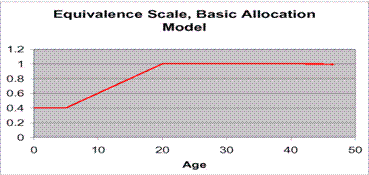
A formula for the scale is:

$\alpha(a)= 1-0.6*D(4<a<20)*((20-a)/16-0.6*D(a<=4)$

where D(x) is a dummy variable equal to 1 when condition x is met. Again, this scale is used to allocate the expenditure for each household j to household member i.

${CFX}_i_j(x)={CFX}_j \alpha(x)/\sum_a \alpha(a) M_j(a)$

where x is the age of the ith household member. Stata programming code for Taiwan is available in the Appendix section.

2.2.2 Public Consumption

Introduction

Public consumption is the value of goods and services individuals receive through the public sector. Public consumption is allocated to individuals based on administrative records and, in some instances, survey data. Like private consumption, public consumption distinguishes education, health, and other public consumption.

Public education consumption consists of two parts: formal and informal education consumption. Formal education consumption is government spending on primary, secondary and higher education levels. The informal education consumption refers to expenditure on culture, religious studies and other types of education. Public health consumption consists of health care purchased by individuals and reimbursed through public programs, health care provided directly to individuals by government clinics and hospitals, and collective services, e.g., health education and preventative programs that are provided to the public at large. Health care purchased by individuals and reimbursed through public programs are also included.

Other public consumption consists of public goods and services, such as defense, justice and police, that are not targeted at particular age groups.

Public Education Consumption

Public formal education consumption by age ${E}^F_g(a)$ is estimated by summing unit cost per student per level ${c}_l$ weighted by the number of students by age in each level ${e}_l(a)$ , i.e. ${E}^F_g= \sum_l {e}_l(a) {c}_l$ , where l is a school level. Unit cost per student at each level of education is estimated by dividing public spending on education at that level by the reported number of students. Unit cost of education within each level is assumed not to vary by age. The number of students by age in each level ${e}_l(a)$ , available from administrative records or, if necessary, tabulated from a census or a household survey.

In addition to public formal education, public informal education consumption by age ${E}^n^f_g(a)$ is estimated by dividing total public informal education consumption by total population by age. Public informal education consumption is not age-targeted, so it is allocated equally to everyone. Public education consumption by age is computed by summing public formal education consumption by age and public informal education consumption by age.

Public Health Consumption

Health care provided directly by government programs must be allocated using administrative records, e.g., patient information; and information about the kinds of health care services being provided (child and maternal health, etc.) Note that health care costs associated with pregnancy and birth are assigned to the mother.

Health care purchased by individuals and reimbursed through public programs are captured in household expenditure surveys, and hence, these age profiles can be estimated using the methods described in the section on private health spending.

Collective health services are allocated on a per capita basis assuming that each individual consumes the same amount of these services.

Public Other Consumption

The per capita age profile of other public consumption is assumed to be constant, i.e., these goods and services are allocated equally to all members of the population.

Treatment of Other Public Individual Consumption

In some countries, especially in European countries, public consumption is classified into two main categories, public collective consumption and public individual consumption. By definition, public collective consumption is the part of public consumption that cannot be allocated to individuals due to its nature, and hence, will be allocated equally to all members of the population. Other public individual consumption is the part of public consumption that can be allocated by age. Publicly provided child day-care services in Finland is an example. These services will be allocated to the beneficiaries of the services.

2.2.3 Labor Income

Introduction

Labor income includes all compensation that is a return to work effort, including labor earnings, employer-provided benefits, taxes paid to the government on behalf of employees, and the portion of entrepreneurial income which is a return to labor.

Compensation of employees includes the value of social benefits provided to workers, including payments to retirees. In principle, compensation should include the imputed value of providing the social benefit to employees. For example, if employees will receive unfunded pension benefits in the future, current compensation should include the imputed value of purchasing an annuity that would provide the future pension. In practice, this is often not possible and the payment of social benefits to current or former workers is counted as current compensation and allocated to current workers.

Compensation also includes compensation to those on paid leave (vacation and sick leave) and hence excluded from labor income calculations. The value of other activities, such as childrearing and other in-home activities, which do not produce market goods or services, is also excluded from labor income calculations.

Labor income includes the portion of entrepreneurial income which is a return to labor. The remaining share of entrepreneurial income is designated as a return to capital, with the share of entrepreneurial income allocated to capital assumed to be the same for each age of worker. In the absence of information to the contrary, we assume that two-thirds of the operating surplus of unincorporated enterprises is labor income. The simple method of allocating two-thirds of mixed income to labor is consistent with the best available evidence on this issue.

Earnings/Fringe Benefits

The age profile of employee compensation is estimated using survey data which reports individual earnings. In general, surveys provide information about wages and salaries of each household member, but do not provide information about employers' social contributions. In the absence of information to the contrary, we assume that employers’ social contribution is a constant proportion of wages and salaries.

Labor Income of the Self-Employed

With few exceptions self-employment income is reported for households rather than individuals. Even in cases where values are reported for individuals, such as in Taiwan, a high percentage is assigned to the household head. Often children or the spouse of the household head are reported as receiving no income and are classified as unpaid family workers. This may lead to under-reporting of the labor income of younger and, often, older household members.

To correct for this problem self-employment income is allocated to family members who are reported as self-employed or as unpaid family workers. The self-employment income of the household is allocated to the members using the age profile of the mean earnings of employees. That is the self-employment income accruing to ith individual in household j (YLSij(x)) is,

${YLS}_i_j(x)= {YLS}_j\gamma(x)$

${\gamma}(x) = w(x){SE}_j(x) / \sum_x w(x){SE}_j(a)$

where x is the age of the ith household member, SEj(x) is the number of people in household j who are self-employed or unpaid family workers of age x, w(x) is the average earnings of employees. Thus, the share of total household self-employment labor income allocated to each household self-employed or unpaid family member of age x is determined.

In this way the total self-employment labor income generated at age x in each household is found, and summing across all households the total self employment labor income generated at age x is found. Stata programming code for Taiwan is available in the Appendix section.

2.2.4 Smoothing

The per capita age profiles are noisy, particularly at ages with relatively few observations, and except as noted below should be smoothed. The following guidelines should be followed:

The per capita education profile should not be smoothed.

Basic components should be smoothed, but not aggregations. For example, private health consumption and public health consumption profiles should be smoothed, but the sum of the two should not be smoothed.

The objective is to reduce sampling variance but not eliminate what may be “real” features of the data. For example,

Public health spending may increase dramatically when individuals reach an age threshold, e.g., 65. This kind of feature of the data should not be smoothed away.

Due to unusual high health consumption by newborns, we tend not to smooth health consumption by age 0. This could be done by including estimated unsmoothed health consumption by newborns to the age profile of smoothed private health consumption by other age groups.

Only adults (usually ages 15 and older) receive income, pay income taxes and make familial transfer outflows. Thus, when we smooth these age profiles, we begin smoothing from the adults age, excluding those younger age group who do not earn income.

However, problem arises when some beginning age group may appear to have negative values for these variables. This could be solved by replacing the negative by the unsmoothed values for the beginning age group.

There are a couple of steps to smoothing the per capita profile. The first step is to create a spreadsheet, which contains unsmoothed age profile and the number of observations for each age. The second step is to use Friedman's SuperSmoother (supsmu function in R) to smooth the per capita profile incorporating the number of observations. The following is the R code to use the command “supsmu”. Suppose “thyl.csv” is the file name (tab delimited excel file format), yl the unsmoothed variable name, and sample is the number of observations for each age in the data. The R programming code is R code;

The alternative smoothing method is “lowess” smoothing. The procedure is found to be unreliable because it does not incorporate sample weights. We recommend that it not be used. However, some researchers may feel more comfortable using the Stata rather than the R program, and would prefer to use the lowess smoothing method. If that is the case, before smoothing the age profile using the lowess command, the survey data are should be adjusted to incorporate the sample weight of each observation. Each observation is duplicated in proportion to its sample weight to produce a representative sample. Then, the lowess command is used to smooth the representative sample.

Illustrative Examples.

After smoothed, the national population age distribution is used to the age profiles to match the macro control total, as described in Aggregate Controls. Figure 2 shows the per capita consumption profile by component for Taiwan in 1998. Most consumption is private rather than public, and in many important areas, food, housing, and clothing, for example, the private sector dominates. The public sector is also important, particularly in education and health. By and large, however, it is private consumption that shapes the consumption side of the lifecycle equation. The sharp increases among children in Taiwan reflect private spending on education.

Smoothing1

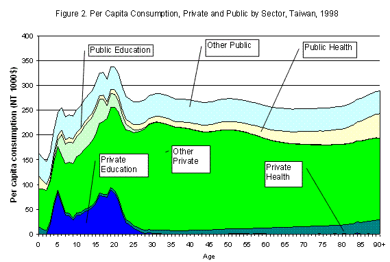
Source: Lee, Lee, and Mason (2008).

Figure 3 presents the per capita labor income profile by component for Finland and the Philippines. Note that, for purposes of comparison, each curve is normalized by dividing it by the unweighted average labor income for ages 30-49. This age range was chosen to exclude younger ages that might be affected by educational enrollments, and older ages that might be affected by retirement. The two labor income profiles are similar, inverse U-shaped. It should come as no surprise that the share of self-employment income is much larger for the Philippines than for Finland. The share of self-employment income is 52% for the Philippines, and 5% for Finland. To the contrary, the share of fringe benefits is much larger for Finland (22%), compared with the Philippines (5%).

Smoothing2

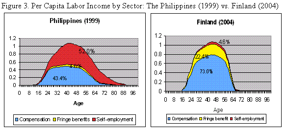
Source: Authors’ calculation.

More information on smoothing is available in 5.3 Other Methods section.

-- Go to next page 3. Public Reallocations

-- Back to Table of Contents